MCMC Introduction

%matplotlib inline
import matplotlib.pyplot as plt
import numpy as np

from py21cmmc import analyse
from py21cmmc import mcmc
import py21cmmc as p21mc

%load_ext autoreload
%autoreload 2

In this notebook we demonstrate how to do the simplest possible MCMC to fit just two astrophysical parameters to a series of coeval brightness temperature boxes without noise, and then visualise the results.

This tutorial will introduce the basic components of using py21cmmc for doing MCMC to fit parameters. For more advanced topics, see the relevant tutorials, guides or FAQs.

p21mc.__version__

'1.0.0dev'

The Structure of 21MCMC

As a bit of a primer, we discuss some of the implementation structure for how likelihoods are actually evaluated in 21CMMC. Understanding this structure will help to identify any issues that may arise, construct useful likelihoods, utilise the various options that the built-in structures have, and eventually to create your own (see XXX for more details of how to do this).

The structure of an MCMC routine in 21CMMC is based on that offered by the cosmoHammer library, but with heavy modifications. This structure is based on a single master LikelihoodComputationChain (let’s just call it the Chain), which houses a number of what we’ll call cores and likelihoods. These are instances of Python classes which can be named arbitrarily (and in principle do not need to be subclassed from any particular object), but follow a minimal API, which we’ll outline shortly. In short, any Chain requires at least one core, and at least one likelihood. Multiples of each are allowed and will work together seamlessly.

Any MCMC should be run using the run_mcmc function in 21CMMC. While the MCMC can be run manually by setting up a Chain with its cores and likelihoods, there are various pitfalls and gotchas associated with this that usually make it easier just to use the in-built function. This function will take a list of cores and likelihoods, along with some specifications of how the MCMC is to proceed, set up a Chain, run the MCMC sampling, and return the Chain object to you.

Thus, almost all of the flexibility of 21CMMC lies in the construction of the various core and likelihood modules.

Core and Likelihood Modules

Let’s briefly discuss these important core and likelihood modules – the philosophy behind them, and what they can and can’t do. We’ll leave a discussion of how to go about implementing your own for another tutorial.

The basic idea behind core and likelihood modules is that the cores are supposed to do the calculations to fill up what is called a context dictionary on every iteration of the MCMC. The likelihoods then use the contents of this context to evaluate a likelihood (this ends up being the sum of the likelihood returned by each likelihood module).

In practice, there is no hard-and-fast limit to the scope of the core or likelihood: the core could evaluate the likelihood itself, store it in the context, and the likelihood could merely access and return it. Likewise, the core could do nothing, and let the likelihood perform the entire calculation.

For practical and philosophical reasons, however there are a few properties of each which dictate how best to separate the work that each kind of module does:

1. All core modules constructively interfere. That is, they are invoked in sequence, and the output of one propagates as potential input to the next. The various quantities that are computed by the cores are not over-written (unless specifically directed to), but are rather accumulated.

2. Conversely, all likelihood modules are invoked after all of the core modules have been invoked. Each likelihood module is expected to have access to all information from the sequency of cores, and is expected not to modify that information. The operation of each likelihood is thus in principle independent of each of the other likelihoods. This implies that the total posterior is the sum of each of the likelihoods, which are considered statistically independent.

3. Due to the first two points, we consider cores as constructive and likelihoods as reductive. That is, it is most useful to put calculations that build data given a set of parameters in cores, and operations that reduce that data to some final form (eg. a power spectrum) in the likelihoods. This is because a given dataset, produced by the accumulation of cores, may yield a number of independent likelihoods, while these likelihoods may be equally valid for a range of different data models (eg. inclusion or exclusion of various systematic effects).

4. Point 3 implies that it is cleanest if all operations that explicitly require the model parameters occur in cores. The reduction of data should not in general be model-dependent. In practice, the current parameters are available in the likelihoods, but we consider it cleaner if this can be separated.

5. In general, as both the cores and likelihoods are used to build a probabilistic model which can be used to evaluate the likelihood of given data, both of their output should in principle be deterministic with respect to input parameters. Nevertheless, one may consider the process as a forward-model, and a forward-model is able to produce mock data. Indeed, 21CMMC adds a framework to the base cosmoHammer for producing such mock data, which are inherently stochastic. A useful way to conceptualize the separation of core and likelihood is to ensure that all stochasticity can in principle be added in the core, and that the likelihood should have no aspect of randomness in any of its calculations. The likelihood should reduce real/mock data in the same way that it reduces model data.

Given these considerations, the core modules that are implemented within 21CMMC perform 21cmFAST simulations and add these large datasets to the context, while the various likelihoods will use this “raw” data and compress it down to a likelihood – either by taking a power spectrum, global average or some other reduction.

Some of the features of cores as implemented in 21CMMC are the following. Each core: * has access to the entire Chain in which it is embedded (if it is indeed embedded), which enables sharing of information between cores (and ensuring that they are consistent with one another, if applicable). * has access to the names of the parameters which are currently being constrained. * is enabled for equality testing with other cores. * has a special method (and runtime parameters) for storing arbitrary data in the Chain on a per-iteration basis (see the advanced MCMC FAQ for more info). * has an optional method for converting a data model into a “mock” (i.e. incorporating a random component), which can be used to simulate mock data for consistency testing.

Some of the features of likelihoods as implemented in 21CMMC are that each likelihood: * also has access to the Chain and parameter names, as well as equality testing, like the cores. * computes the likelihood in two steps: first reducing model data to a “final form”, and then computing the likelihood from this form (eg. reducing a simulation cube to a 1D power spectrum, and then computing a \(\chi^2\) likelihood on the power spectrum). This enables two things: (i) production and saving of reduced mock data, which can be used directly for consistency tests, and (ii) the ability to use either raw data or reduced data as input to the likelihood. * has methods for loading data and noise from files. * has the ability to check that a list of required_cores are loaded in the Chain.

Running MCMC

Enough discussion, let’s create our core and likelihood. In this tutorial we use a single core – one which evaluates the coeval brightness temperature field at an arbitrary selection of redshifts, and a single likelihood – one which reduces the 3D field(s) into a 1D power spectrum/spectra and evaluates the likelihood based on a \(\chi\)-square fit to data.

core = p21mc.CoreCoevalModule( # All core modules are prefixed by Core* and end with *Module
    redshift = [7,8,9],          # Redshifts of the coeval fields produced.
    user_params = dict(       # Here we pass some user parameters. Also cosmo_params, astro_params and flag_options
        HII_DIM = 50,         # are available. These specify only the *base* parameters of the data, *not* the
        BOX_LEN = 125.0       # parameters that are fit by MCMC.
    ),
    regenerate=False          # Don't regenerate init_boxes or perturb_fields if they are already in cache.
) # For other available options, see the docstring.

# Now the likelihood...
datafiles = ["data/simple_mcmc_data_%s.npz"%z for z in core.redshift]

likelihood = p21mc.Likelihood1DPowerCoeval(  # All likelihood modules are prefixed by Likelihood*
    datafile = datafiles,                   # All likelihoods have this, which specifies where to write/read data
    noisefile= None,                        # All likelihoods have this, specifying where to find noise profiles.
    logk=False,                             # Should the power spectrum bins be log-spaced?
    min_k=0.1,                              # Minimum k to use for likelihood
    max_k=1.0,                              # Maximum ""
    simulate = True,                        # Simulate the data, instead of reading it in.
                                            # will be performed.
) # For other available options, see the docstring

Now we have all we need to start running the MCMC. The most important part of the call to run_mcmc is the specification of params, which specifies which are the parameters to be fit. This is passed as a dictionary, where the keys are the parameter names, and must come from either cosmo_params or astro_params, and be of float type. The values of the dictionary are length-4 lists: (guess, min, max, width). The first specifies where the best guess of the true value lies, and the initial walkers will be chosen around here. The min/max arguments provide upper and lower limits on the parameter, outside of which the likelihood will be -infinity. The width affects the initial distribution of walkers around the best-guess (it does not influence any kind of “prior”).

Finally, the model_name merely affects the file name of the output chain data, along with the datadir argument.

model_name = "SimpleTest"

chain = mcmc.run_mcmc(
    core, likelihood,        # Use lists if multiple cores/likelihoods required. These will be eval'd in order.
    datadir='data',          # Directory for all outputs
    model_name=model_name,   # Filename of main chain output
    params=dict(             # Parameter dict as described above.
        HII_EFF_FACTOR = [30.0, 10.0, 50.0, 3.0],
        ION_Tvir_MIN = [4.7, 4, 6, 0.1],
    ),
    walkersRatio=3,         # The number of walkers will be walkersRatio*nparams
    burninIterations=0,      # Number of iterations to save as burnin. Recommended to leave as zero.
    sampleIterations=150,    # Number of iterations to sample, per walker.
    threadCount=6,           # Number of processes to use in MCMC (best as a factor of walkersRatio)
    continue_sampling=False  # Whether to contine sampling from previous run *up to* sampleIterations.
)

/home/steven/miniconda3/envs/21CMMC/lib/python3.7/site-packages/powerbox/dft.py:121: UserWarning: You do not have pyFFTW installed. Installing it should give some speed increase.
  warnings.warn("You do not have pyFFTW installed. Installing it should give some speed increase.")
2019-11-15 12:25:59,295 | WARNING | likelihood.py::_write_data() | File data/simple_mcmc_data_7.npz already exists. Moving previous version to data/simple_mcmc_data_7.npz.bk
2019-11-15 12:25:59,297 | WARNING | likelihood.py::_write_data() | File data/simple_mcmc_data_8.npz already exists. Moving previous version to data/simple_mcmc_data_8.npz.bk
2019-11-15 12:25:59,298 | WARNING | likelihood.py::_write_data() | File data/simple_mcmc_data_9.npz already exists. Moving previous version to data/simple_mcmc_data_9.npz.bk

Analysis

Accessing chain data

The full chain data, as well as any stored data (as “blobs”) is available within the chain as the samples attribute. If access to this “chain” object is lost (eg. the MCMC was run via CLI and is finished), an exact replica of the store object can be read in from file. Unified access is provided through the get_samples function in the analyse module. Thus all these are equivalent:

samples1 = chain.samples

samples2 = analyse.get_samples(chain)

samples3 = analyse.get_samples("data/%s"%model_name)

# Equivalent:
# samples = analyse.get_samples("data/%s"%model_name)

print(np.all(samples1.accepted == samples2.accepted))
print(np.all(samples1.accepted == samples3.accepted))

True
True

Do note that while the first two methods return exactly the same object, occupying the same memory:

samples1 is samples2

True

this is not true when reading in the samples from file:

print(samples1 is samples3)
del samples3; samples=samples1 # Remove unnecessary memory, and rename to samples

False

Several methods are defined on the sample object (which has type HDFStore), to ease interactions. For example, one can access the various dimensions of the chain:

niter = samples.size
nwalkers, nparams = samples.shape

We can also check what the parameter names of the run were, and their initial “guess” (this is the first value passed to the “parameters” dictionary in run_mcmc:

print(samples.param_names)
print([samples.param_guess[k] for k in samples.param_names])

('HII_EFF_FACTOR', 'ION_Tvir_MIN')
[array([30.]), array([4.7])]

Or one can view how many iterations were accepted for each walker:

samples.accepted, np.mean(samples.accepted/niter)

(array([106,  98,  95, 105, 109, 109]), 0.6911111111111111)

We can also see what extra data we saved along the way by getting the blob names (see below for more details on this):

samples.blob_names

('k_z7', 'delta_z7', 'k_z8', 'delta_z8', 'k_z9', 'delta_z9')

Finally, we can get the actual chain data, using get_chain and friends. However, this is best done dynamically, as the samples object itself does not hold the chain in memory, rather transparently read it from file when accessed.

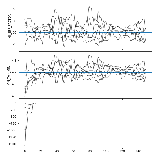
Trace Plot

Often, for diagnostic purposes, the most useful plot to start with is the trace plot. This enables quick diagnosis of burnin time and walkers that haven’t converged. The function in py21cmmc by default plots the log probability along with the various parameters that were fit. It also supports setting a starting iteration, and a thinning amount.

analyse.trace_plot(samples, include_lnl=True, start_iter=0, thin=1, colored=False, show_guess=True);

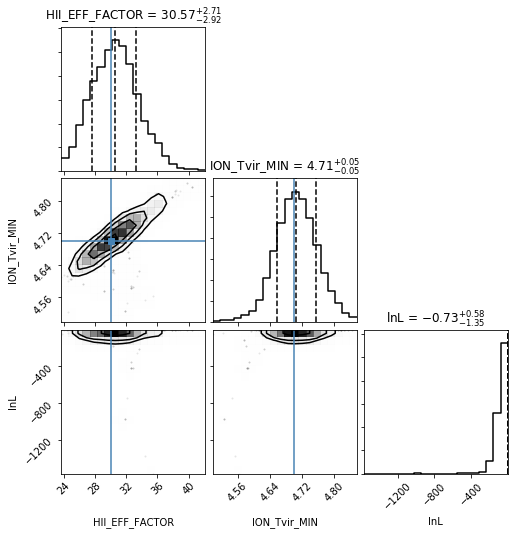
Corner Plot

One of the most useful plots to come out of an MCMC analysis is the “corner” plot, which shows the correlation of each parameter with every other parameter. The function in py21cmmc will by default also show the original “guess” for each parameter as a blue line, and also show the log-likelihood as a psuedo-“parameter”, though this can be turned off.

samples.param_guess

array([(30., 4.7)],
      dtype=[('HII_EFF_FACTOR', '<f8'), ('ION_Tvir_MIN', '<f8')])

analyse.corner_plot(samples);

Model Comparison Plot

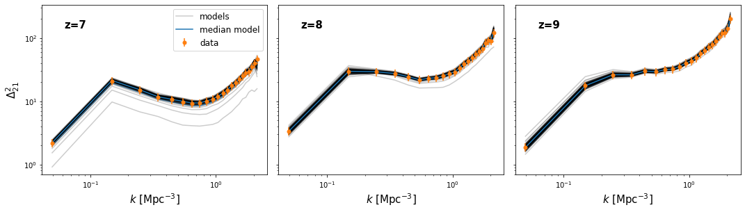
Another plot of interest is a “model comparison” plot – i.e. comparing the range of outputted models to the data itself. These will differ significantly depending on the kind of data produced by the likelihood function, and thus they depend also on the actual data used. We thus do not provide a general function for plotting this. We do however show how one might go about this task in the function below.

First, however, we show how one might interact with the data and saved models/blobs.

To extract all blob data from the samples:

blobs = samples.get_blobs()

For simplicity, let’s extract each kind of blob from the blob structured array:

k = blobs['k_z7']
model_power = blobs['delta_z7'], blobs['delta_z8'], blobs['delta_z9']

print(k.shape, model_power[0].shape)
nk = k.shape[-1]

(150, 6, 22) (150, 6, 22)

Here we notice that k should be the same on each iteration, so we take just the first:

print(np.all(k[0] == k[1]))
k = k[0]

True

Finally, we also want to access the data to which the models have been compared. Since we have access to the original likelihood object, we can easily pull this from it. However, we equivalently could have read it in from file (this file is not always present, only if datafile is present in the likelihood constructor):

p_data = np.array([d['delta'] for d in likelihood.data])
k_data = np.array([d['k'] for d in likelihood.data])

# Equivalent
# data = np.genfromtxt("simple_mcmc_data.txt")
# k_data = data[:,0]
# p_data = data[:,1:]

Now, let’s define a function which will plot our model comparison:

def model_compare_plot(samples, p_data, k_data, thin=1, start_iter=0):
    chain = samples.get_chain(thin=thin, discard=start_iter, flat=True)
    blobs = samples.get_blobs(thin=thin, discard=start_iter, flat=True)

    k = blobs['k_z7'][0]
    model_power = [blobs[name] for name in samples.blob_names if name.startswith("delta_")]

    print(k.shape)

    nz = len(model_power)
    nk = k.shape[-1]

    fig, ax = plt.subplots(1, nz, sharex=True, sharey=True, figsize=(6*nz, 4.5),
                          subplot_kw={"xscale":'log', "yscale":'log'}, gridspec_kw={"hspace":0.05, 'wspace':0.05},
                          squeeze=False)

    for i in range(nz):
        this_power = model_power[i]
        this_data = p_data[i]

        label="models"

        for pp in this_power:
            ax[0,i].plot(k, pp, color='k', alpha=0.2, label=label, zorder=1)
            if label:
                label=None

        mean = np.mean(this_power, axis=0)
        std = np.std(this_power, axis=0)
        md = np.median(this_power, axis=0)

        ax[0,i].fill_between(k, mean - std, mean+std, color="C0", alpha=0.6)
        ax[0,i].plot(k, md, color="C0", label="median model")

        ax[0,i].errorbar(k_data, this_data, yerr = (0.15*this_data), color="C1",
                     label="data", ls="None", markersize=5, marker='o')

        ax[0,i].set_xlabel("$k$ [Mpc$^{-3}$]", fontsize=15)
        ax[0,i].text(0.1, 0.86, "z=%s"%core.redshift[i], transform=ax[0,i].transAxes, fontsize=15, fontweight='bold')

    ax[0,0].legend(fontsize=12)
    #plt.ylim((3.1e2, 3.5e3))


    ax[0,0].set_ylabel("$\Delta^2_{21}$", fontsize=15)

#plt.savefig(join(direc, modelname+"_power_spectrum_plot.pdf"))

model_compare_plot(samples, p_data, k_data[0], thin=10)

(22,)